Mayavi — Plotting vectors

Mayavi is the 3D plotting module for Python, which is very straight forward to use regarding point data, but when it comes to vector data one has to regard the data type required by the function quiver3d().

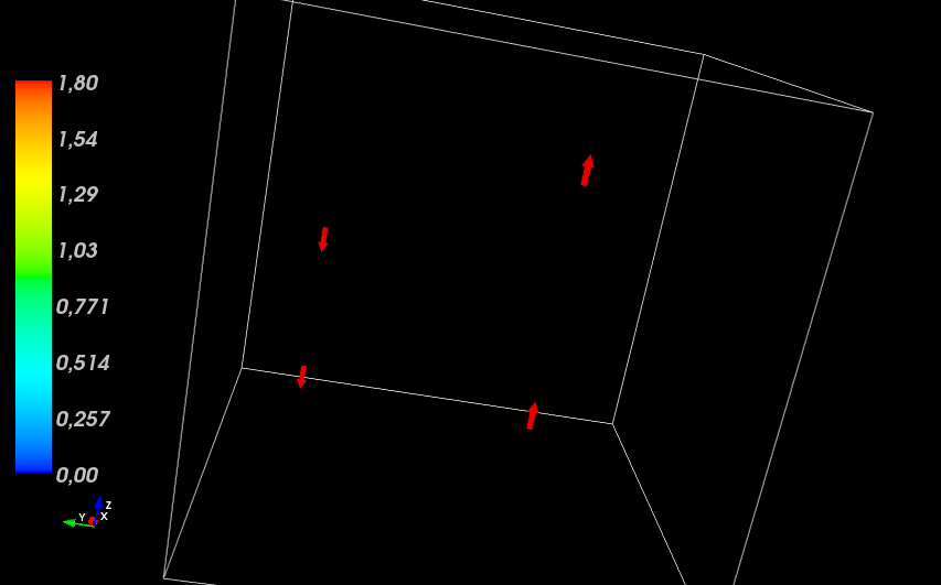
Some time ago I was asked to give a short intro on how to plot a set of vectors at certain positions in Mayavi as shown in the image above.

The solution

Mayavi's quiver3d() function specifically requires at least three 3D NumPy arrays as its basic idea is to plot a vector field on a cubic domain. So the first thing to do is define the coordinate system

#!/usr/bin/env python

import numpy
import mayavi.mlab

x,y,z = numpy.mgrid[-0.1:0.9:32j,-0.1:0.9:32j,-0.1:0.9:32j]

m = numpy.array([
    numpy.zeros_like(x),
    numpy.zeros_like(y),
    numpy.zeros_like(z)
])

The variable x contains only the x-value of the cubic domain, the variable y contains only the y-value and so on. For those new to Mayavi the third parameter in each argument of mgrid (e.g. "32j") in line 6 defines the number of data points in each direction. Then we need a corresponding data structure for the magnetic moments — the variable m. Instead of using components like x, y and z I prefer one 4-dimensional variable, if possible, such that e.g. m[0] is the 3D cube containg x values. By default I choose zero values.

The tricky part now is to set the vector components in the variable m to desired values at the desired position. Therefor one has to get the value for the corresponding index first.

X = numpy.argmin(abs(x[:,0,0]-0.25))
Z = numpy.argmin(abs(x[:,0,0]-0.136))

m[0,X,X,Z]=0
m[1,X,X,Z]=0
m[2,X,X,Z]=1.8

In other words one looks for the index with value closest to the desired value. Having the indices one can set the vector components in the variable m. As you might have noticed the x and y coordinates and components are equal in this example. Now for some more vectors:

Z = numpy.argmin(abs(x[:,0,0]-0.635))
m[0,X,X,Z]=0
m[1,X,X,Z]=0
m[2,X,X,Z]=1.8

X = numpy.argmin(abs(x[:,0,0]-0.75))
Z = numpy.argmin(abs(x[:,0,0]-0.3652))
m[0,X,X,Z]=0
m[1,X,X,Z]=0
m[2,X,X,Z]=-1.8

Z = numpy.argmin(abs(x[:,0,0])-0.866)
m[0,X,X,Z]=0
m[1,X,X,Z]=0
m[2,X,X,Z]=-1.8

Having defined all our vectors we can finally conclude the example by plotting the "vector field". As mentioned earlier quiver3d() requires 3D-arrays; so we have to pass the components of m to the function.

mayavi.mlab.quiver3d(x,y,z,m[0],m[1],m[2])
mayavi.mlab.outline()
mayavi.mlab.colorbar()
mayavi.mlab.show()

For a fancier output I have added a wireframe outline and a colorbar legend. To get the actual output one finally needs the show() function. Et voila!