Integration over a n-dim. array for each element of a n-dim. result-array
In numerical calculations a well known "problem" can be the integration or summation of an entire array when the result of this summation is required for each field of an equally large array, e.g. in the calculation of the electro static potential of a given charge distribution:

The Problem
Intuitivaly one would require n nested loops for each dimension of the array representing Φ(x) and another n loops nested within for Q -- thus one would need to write 2*n nested loops in order to get the full sum over Q for each point in Φ.
Especially in Python this approach is rather slow. Even the attempt of writing an appropriate subroutine in C or with Cython will not be the sole measure of writing an efficient code.
The solution
One can get rid of the n nested loops for Q when exploiting the mathematical properties of NumPy arrays. Instead one can write the term in the divisors of equations (1) and (2) as the simle difference of a scalar represing the current field of Φ and an n-dimensional array specifying all possible x-values for Q. This is quite elegant as one will need this large arrays, too, when the data shall be plotted with correct numbering of the axes.
The above mentioned logic can be found in lines 14 - 22 of the following example. In order to use more CPU cores, if present, for the calculation the nested loops are located within a Python-Thread.
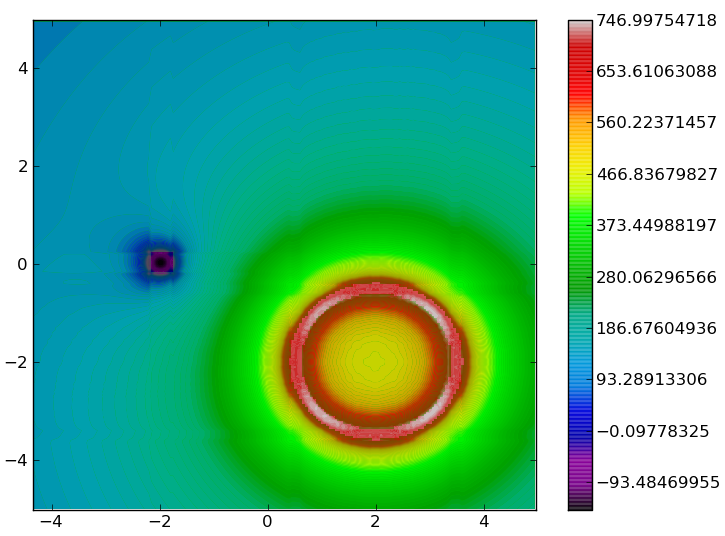
In lines 33 - 47 one can find a charge density distribution describing a rectangle carrying chanrges on its border. The commented lines 68 and 74 would calculate the electric field from the potential and add a quiver plot to the figure, if uncommented
#!/usr/bin/env python
# -*- coding: utf8 -*-

import pylab
import threading

class MyThread(threading.Thread):
    def __init__(self,y_lower,y_upper):
        threading.Thread.__init__(self)
        self.y_lower= y_lower
        self.y_upper = y_upper

    def run(self):
        for xi in range(len(x)):
            for yi in range(self.y_lower,self.y_upper):
                P[yi,xi] = pylab.sum(
                    pylab.select(
                        [(x[xi]-X)*(x[yi]-Y)==0,],
                        [0,],
                        Q/pylab.sqrt((x[xi]-X)**2+(x[yi]-Y)**2)
                    )
                )

dx = .05
x = pylab.arange(-5,5,dx)
X,Y = pylab.meshgrid(x,x)

# Homogeneous charge density
Q = pylab.zeros_like(X)
Q = pylab.select([abs(X+2)<4*dx,],[pylab.select([abs(Y)<4*dx,],[-1,],0),],Q)
#Q += pylab.select([abs(X+.5)<.3,],[pylab.select([abs(Y)<.33],[-1,],0),],Q)

# Sharp rectangular charge density
#Q = pylab.zeros_like(X)
#Q[40,31:70] = 1
#Q[41:45,30] = 1
#Q[41:45,70] = 1
#Q[45,31:70] = 1

#Q[60,46:54] = -1
#Q[61:62,45] = -1
#Q[61:62,54] = -1
#Q[62,46:54] = -1

# Sharp circular charge density
#Q = pylab.zeros_like(X)
Q = pylab.select([abs((X-2)**2+(Y+2)**2-(1.5)**2)<pylab.sqrt(2*dx)],[1],Q)

P = pylab.zeros_like(X)

threads = []
dy = 4
for i in range(dy):
    y_lower = int(len(x)/dy*float(i))
    y_upper = int(len(x)/dy*float(i+1))
    t = MyThread(y_lower,y_upper)
    threads.append(t)
    t.start()

if y_upper < len(x):
    t = MyThread(y_upper,len(x))
    threads.append(t)
    t.start()

for t in threads:
    t.join()

#E = pylab.gradient(P)
pylab.gray()
pylab.pcolormesh(X,Y,Q)
pylab.spectral()
pylab.contourf(X,Y,P,levels=pylab.linspace(P.min(),P.max(),125),alpha=.8))
pylab.colorbar()
#pylab.quiver(X,Y,E[1],E[0],pivot='middle',alpha=.5,color='gray')
pylab.show()

Figure 1: Resulting electro static potential for
a ring with positive charges (right bottom) and
a square with negative charge (left top).
Variation
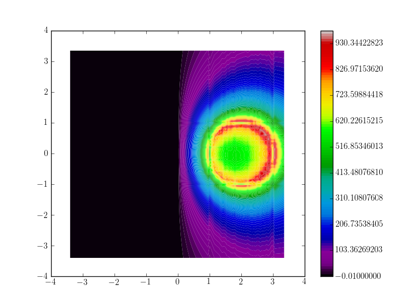
A little variation of the above problem could contain an a grounded electrode, e.g. at the plane x=0. This problem is treated with image charges behind the grounded plane (see [1]).
#!/usr/bin/env python
# -*- coding: utf8 -*-

import pylab
import threading

class MyThread(threading.Thread):
    def __init__(self,y_lower,y_upper):
        threading.Thread.__init__(self)
        self.y_lower= y_lower
        self.y_upper = y_upper

    def run(self):
        for xi in range(len(x)):
            for yi in range(self.y_lower,self.y_upper):
                P[yi,xi] = pylab.sum(
                    pylab.select(
                        [(x[xi]-X)*(x[yi]-Y)==0,],
                        [0,],
                        (Q+Q_shadow)/pylab.sqrt((x[xi]-X)**2+(x[yi]-Y)**2)
                    )
                )

dx = .05
x = pylab.arange(-3.4,3.4,dx)
X,Y = pylab.meshgrid(x,x)
Q_shadow = pylab.zeros_like(X)
Q = pylab.zeros_like(X)

# Sharp circular charge density
P_ini = pylab.zeros_like(X)
x0, y0, r =2, 0, 1
Q = pylab.select([abs((X-x0)**2+(Y-y0)**2-r**2)<(5*dx)**2],[5],[0])
Q_shadow = -1*pylab.fliplr(Q)

P = pylab.zeros_like(X)
threads = []
dy = 4
for i in range(dy):
    y_lower = int(len(x)/dy*float(i))
    y_upper = int(len(x)/dy*float(i+1))
    t = MyThread(y_lower,y_upper)
    threads.append(t)
    t.start()

if y_upper < len(x):
    t = MyThread(y_upper,len(x))
    threads.append(t)
    t.start()

for t in threads:
    t.join()

P = pylab.select([X>0],[P],[0])

pylab.spectral()
pylab.contourf(X,Y,P,levels=pylab.linspace(P.min()-1e-2,P.max(),96),alpha=1)
pylab.colorbar()
pylab.show()

Figure 2: Electrostatic potential of a charged ring
in front of a grounded plane at x=0
The elegant solution
There is a variety of problems which require solutions like eq. (1) and (2), but in the case of electrostatics there is a way to regard grounded objects -- or in more general boundary conditions -- in an elegant way: Solving the Lapace- or Poisson equation.
Usage of a PDE (partial differential equation) solver based on e.g. finite elements such as FiPy allows us to define boundary conditions (e.g. grounded plate, electrode on a given potential or charge distribution). Thus one has not to determine the shape of image charges behind a grounded surface.
References
- Dall’Agnol, F. F. & Mammana, V. P.
Solution for the electric potential distribution produced by sphere-plane electrodes using the method of images
Revista Brasileira de Ensino de Fisica, 2009, 31, 3503