Visualize the Orbitals of the Hydrogen atom in 3D

Description

At first we need to import the module providing the required data structures (numpy) and mathematical tools (scipy.misc, scipy.special). To obtain a nice 3-dimensional plot we import enthought.mayavi.mlab.

As the solutions to the Schrödinger equation in the case of the hydrogen atom are rotationally symmetric, we define the spherical coordinates (r,theta,phi) as functions of the cartesian coordinates (x,y,z), which form the grid (numpy.ogrid!) for this plot. Now that we work in spherical coordinates we can define the wave function (solution to Schrödinger equation) as the product of a radial function, which depends on r and two quantum numbers n,l, and a spherical harmonic, which depends on the angles theta,phi and two quantum numbers. As the values of this wave function can become complex we define a function to determine the squared absolute value of the wave function, which is also a measure for the probability of finding an electron at any point.

The variable mask as defined in the comment section would cause the wavefunction in the plot to appear like a pie which is missing a slice.

The mlab.figure() call is not required unless we want multiple windows with plots.

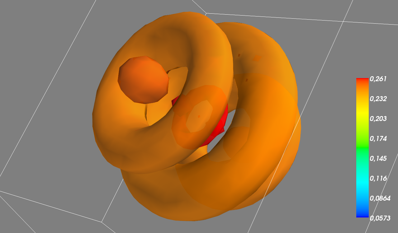
Using three loops we iterate over all atomic orbitals from 1s to 3d and add its contour plot of its squared value to the output. Finally we also add a colorbar (on the right) and a frame box around the orbitals.

At the end we tell Python to show (mlab.show()) us the result, which can take some time as we did not bother to use more than one CPU for this task.

Results

Figure 1: Output of script as shown above.

Figure 2: Output of script, which only displays the 3d orbitals.
In addition the mask variable shown in the comment area was used.

Source Code

#!/usr/bin/env python

import numpy
import scipy.special
import scipy.misc
from enthought.mayavi import mlab

r = lambda x,y,z: numpy.sqrt(x**2+y**2+z**2)
theta = lambda x,y,z: numpy.arccos(z/r(x,y,z))
phi = lambda x,y,z: numpy.arctan(y/x)
#phi = lambda x,y,z: numpy.pi+numpy.select(
#	[x>0, x==0, x<0],
#	[
#		numpy.arctan(y/x),
#		.5*numpy.pi*numpy.sign(y),
#		numpy.arctan(y/x)+numpy.pi*numpy.sign(y)]
#)
a0 = 1.
R = lambda r,n,l: (2*r/n/a0)**l * numpy.exp(-r/n/a0) * scipy.special.genlaguerre(n-l-1,2*l+1)(2*r/n/a0)
WF = lambda r,theta,phi,n,l,m: R(r,n,l) * scipy.special.sph_harm(m,l,phi,theta)
absWF = lambda r,theta,phi,n,l,m: abs(WF(r,theta,phi,n,l,m))**2

x,y,z = numpy.ogrid[-24:24:55j,-24:24:55j,-24:24:55j]

mlab.figure()

#mask = numpy.select([theta(x,y,z)>numpy.pi/3.],[numpy.select([abs(phi(x,y,z))<numpy.pi/3.],[numpy.nan],default=1)],default=1)
mask = 1

for n in range(2,3):
	for l in range(1,n):
		for m in range(-l,l+1,1):
			w = absWF(r(x,y,z),theta(x,y,z),phi(x,y,z),n,l,m)
			mlab.contour3d(w*mask,contours=6,transparent=True)

mlab.colorbar()
mlab.outline()
mlab.show()